Four Parameter Logistic Regression
You have been asked to perform an ELISA to detect a molecule in a biologic matrix. All you have to do is test the sample using any number of commercially available kits. Maybe you will even develop your own assay. No problem. You’ll probably want to also determine the quantity of the material you have detected. This is where things can get interesting.
In order to determine a quantity of something you will need to compare your sample results to those of a set of standards of known quantities. The standards, in your assay, should be tested at a range of concentrations that yields results from essentially undetectable to maximum signal. This set of data for the standards allows one to “fit” a statistical model and generate a predicted standard curve. You can think of the standard curve as the ideal data for your assay. Once the standard curve is generated it is relatively easy to see where on the curve your sample lies and interpolate a value. Let’s look at a simple model to discuss how to “fit” a curve and a more complex, “biologically relevant” model to start applying what we know.
Choosing a model really depends on a thorough understanding of what it is that you are measuring (see How to Choose and Optimize ELISA Reagents and Procedures). For now, I will talk about two models:
Linear Regression
To start let’s look at the simplest model, known as a linear regression:

In this model we have the following:
y = the dependent variable (i.e. what you measure as the signal)
x = the independent variable (i.e. what you control, such as, dose, concentration, etc.)
m = the slope of the fitted line
c = the intercept of the dependent axis
If you have made it past algebra in school you have most likely encountered this model. The goal is to determine values of m and c which minimize the differences (residuals) between the observed values (i.e. your data) and the predicted values (i.e. the fitted curve). To check the predicted fit of the line one usually calculates all the residuals (observed – predicted) and sums all the differences. The smaller the sum the better the data fit the predicted curve. However, since some observed values will likely be above the fitted curve and some below you will get positive and negative residuals. Summing these is not very useful, as even a random set of data points may generate residuals that sum close to zero. To get around this you should square each of the residuals, which render all the values positive, then sum them. This is known as the sum of squares (SSq). The smaller the SSq, the closer the observed values are to the predicted, the better the model predicts your data. The good news is that linear regression is pretty easy. The bad news is that linear regression is seldom a good model for biological systems.
Four Parameter Logistic (4PL) Regression
This leads us to another model of higher complexity that is more suitable for many biologic systems. This model is known as the 4 parameter logistic regression (4PL). It is quite useful for dose response and/or receptor-ligand binding assays, or other similar types of assays. As the name implies, it has 4 parameters that need to be estimated in order to “fit the curve”. The model fits data that makes a sort of S shaped curve. The equation for the model is:
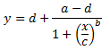
Of course x = the independent variable and y = the dependent variable just as in the linear model above. The 4 estimated parameters consist of the following:
a = the minimum value that can be obtained (i.e. what happens at 0 dose)
d = the maximum value that can be obtained (i.e. what happens at infinite dose)
c = the point of inflection (i.e. the point on the S shaped curve halfway between a and d)
b = Hill’s slope of the curve (i.e. this is related to the steepness of the curve at point c).
The rearranged equation to solve x is:
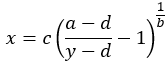
Note that the a and d values might be flipped, however, a and d will always define the upper and lower asymptotes (horizontals) of the curve. a and d are the same units at y. The curve can only be used to calculate concentrations for signals within a and d. Samples outside the range of the determined a and d cannot be calculated.
This model is a little trickier than the linear regression model above. If you topped out at algebra you may not have seen this curve, but rest assured, a little algebra is all you will need to solve for x, given your data y. You may now be thinking what do I do with a, b, c, and d. Lucky for you there are many excellent curve fitting programs out there that will do the heavy lifting for you. MyAssays will take your data and estimate some initial values for these parameters and hone in on the best fit using the least squares method described above. Best of all you can use MyAssays to do this for any of the assays that are offered on our web site. In the end a nice neat report is produced that documents the best fit curve, the obtained parameters, and your interpolated data values.
4PL and IC50/EC50/ED50
A common requirement is to calculate IC50/EC50/ED50 from the fit. There are actually two ways to do this depending on what you consider IC50/EC50/ED50 to be:
Firstly, the midpoint of the sigmoid of the 4PL is equal to the c coefficient of the 4PL. In this case you can simply look at the calculated c coefficient. Use this method if you consider the midpoint of the sigmoid to be equal to IC50/EC50/ED50. Mathematically this is the case as it is the x point at exactly half way between the two horizontal asymptotes.
Alternatively, if the response is measured between 0 and 100% and you consider IC50/EC50/ED50 to be where y = 50 then you can calculate where y = 50 using the equation to solve x (above), substituting in the calculated coefficients.
Tips
For an overview of available 4PL curve-fitting tools for ELISA, please see ELISA Data Analysis Tools for Performing 4PL (and 5PL Fits)
Here are a few things to remember for each assay run:
• Look at your data, no matter whose curve fitting software you utilize. Good old observation can tell you a lot about what is going on in your assay. The MyAssays Interactive Chart displays your chart and can be used to mark outliers to exclude.
• Make sure your curve moves in the correct direction. If you are measuring direct binding then your signal should start low, at a low concentration of test agent, and curve upwards as you increase dose. A competitive binding assay or toxicity assay will start with a high signal, at low concentrations of test agent, and the signal will decrease as you add more and more sample.
• Running replicate samples is always a good idea. Replicates provide more robustness and and visualizing the results will let you know if the samples are performing consistently. The MyAssays Layout Editor can be used to specify how your replicates are arranged.
• Additional statistical methods to assure assay consistency across runs are available and will be discussed in a later article. A MyAssays Report typically provides a variety of relevant statistical information.
Let MyAssays help you document your hard work within and across assays. Data analysis and quality assurance were never easier.
To calculate concentrations using Four Parameter Logistic Regression for a typical ELISA try https://www.myassays.com/four-parameter-logistic-curve.assay
Written by James E. Drummond Ph.D
Edited by Darren Cook